Step2: Selection of individuals
Taking into account all the information coming from the previous tables, we can select individuals for producing the next generation.
1. Methods for selection
In OptiMAS, three different ways are possible to select individuals:
Manual selection: selection of individuals based on your own judgment (see Fig. 15). In the step 1 window (molecular score table), select plants via click and drag selection (or simple click + Ctrl) > Press Right click > Add to list... > Selection of your list (can be renamed by double-click) > Ok.

Figure 15: manual selection of individuals added to a list
Individuals are selected manually (a) and then added to a list of your choice (b). This new list can be accessed through the Step 2 interface (c), see above. Names of lists can be modified by the user at all steps (by double clicking on the name of the list one wants to modify).
The two next options are initiated by clicking on the Step 2 icon.
Truncation selection (TS): individuals can be ranked automatically based on four possible criteria: Molecular Score (MS), Weighted MS, Utility Criterion (MS_UC), Index (if computed). The Nsel first sorted individuals are selected to generate the next population. e.g. Nsel = 10, Criterion = MS, List = List2_Truncation_MS_Selection, Option: Cycle = C2 (last cycle), then press Run. A second list can be created by doing the same with Criterion = Weight and List = List3_Truncation_Weight_Selection. The list(s) of selected individuals will appear on the "Selection" page (see Fig. 16).
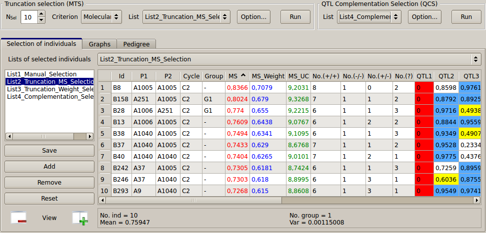
Figure 16: truncation selection based on three criteria (MS, Weighted MS and Utility Criterion)
QTL complementation selection (QCS): takes into account complementarities between candidate individual(s) regarding the favorable alleles they carry (see figures below). It aims at preventing the loss of rare favorable allele(s) (Hospital et al., 2000). This option is important when a high number of QTL is considered. This option completes an initial list with supplementary individuals bringing the complementary alleles. Note that the same name will be kept after complementation.
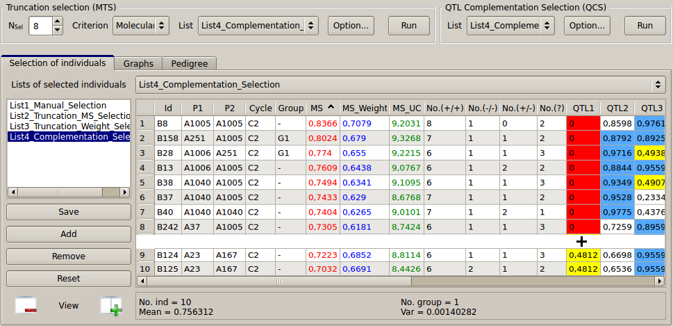
Figure 17: QTL complementation selection
As an example, create a first version of "List4_Complementation_Selection" by applying the “Truncation Selection” based on the MS (Nsel = 8, Criterion = MS, List = List4_Complementation_Selection, Option: Cycle = C2 then press “Run”).
Eight individuals (B8... B242, see Fig. 17) are selected at this step. The colored view points that we are losing the favorable allele for QTL 1 (in red, QTL1 = 0 for all individuals). To complete the list with the QCS procedure, select the "List4_Complementation_Selection” in the QCS section. Click on the QCS "Option..." button to set up the parameters shown in Fig. 18 (on the left side) and press “Apply”. The result appears in a pop-up window (on the right).
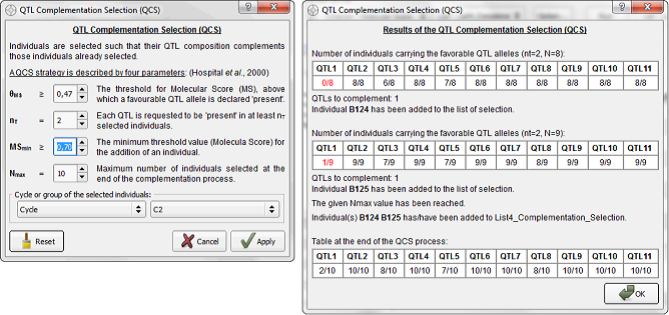
Figure 18: QTL complementation selection algorithm with parameters
In this example, QCS adds two candidates such that their QTL composition complements those eight individuals already selected (see Fig 17 & 18).
The QCS is described by five parameters:
θMS: corresponds to the MS QTL threshold (QTLx > 0.47 by default), above which a favorable QTL allele is declared "present". In this case and depending on the threshold value, not only individuals considered as homozygous for the favorable allele at QTL position will be taken into account (e.g. heterozygous individuals, see Fig. 17, in yellow).
nT: means that each QTL favorable allele is requested to be "present" in at least nT selected individuals (here nT = 2).
MSmin: the minimum threshold value (MSmin ≥ 0, by default) for the addition of an individual. In this example, individuals with MS (genetic value) < 0.7 are not considered.
Nmax: the maximum number of individuals selected at the end of the QCS process. Here, up to two individuals will be added to the final subset of selected individual (Nmax = 10).
Cycle/Group: optional information regarding the generation of selection or another classification criterion in the programme (e.g. first cycle, second cycle, F2, F4, subprogrammes, families, etc). "C2" (cycle 2) was selected instead of "None" (no selection, by default) in order to select individuals that belong to the last cycle of selection.
This approach can be applied to any predefined list (including the possibility to consider an empty list). In this example, the first eight individuals (N0’= 8) were selected via the truncation selection (based on the MS criterion). Then: (i) the QTL for which the favorable alleles are "present" in fewer than nt selected individuals are identified (see Fig. 18, in red); (ii) among the remaining individuals (belonging to Cycle), taken in order of decreasing MS (with MS ≥ MSmin), OptiMAS searches for the individual having favorable alleles "present" at the largest number of those QTL identified in (i). This individual is added to the subset of selected individuals (i.e. N = N0’ + 1). Steps (i) and (ii) are iterated until either of the following conditions is met: favorable alleles at all QTL are present in at least nt individuals of the selected subset, or the number of individuals in the selected subset reaches the given Nmax value, or it is not possible to find an individual in step (ii).
Note that in step (ii), MS is a secondary criterion; individuals are taken based on their ability to complement the subset of already selected individuals. Thus, with the present set of parameters, two individuals (B124, B125) have been added to the selected list (see more details on the right side of Fig. 18).
2. Display and comparison of lists of selected individuals
The different lists of selected individuals can be compared in two parallel tables (see below) displayed by default (which can be reduced to one list by clicking on the "-" button).
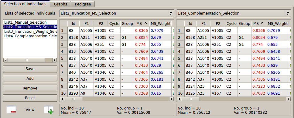
Figure 19: comparison between lists of selected individuals (via tables)
If we compare the two lists of ten individuals selected via the MS (on the left) and QCS (on the right), we can see that the two last individuals (B246 and B293) are replaced by B124 and B125 in the QCS list. The selection of these two individuals will bring two more unfavorable alleles (QTL5 and QTL8 in red, not presented in Fig. 19) in the next generation. Note that individuals can be deleted from a list (right click on the selected individuals and press the “delete...” button). They also can be copied from one list to the other by "drag and drop".
The different lists of individuals can also be compared via the Graphs section window (click on the Graphs tab, see Fig. 20).
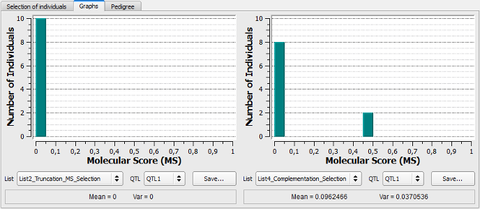
Figure 20: comparison between lists of selected individuals (via graphs)
This example shows that use of truncation selection based on MS leads to the selection of individuals all carrying the unfavorable allele at QTL1 (see above, histogram on the left). On the right side, the two individuals (B124, B125) added via the QCS procedure are observed with a MS comprised between 0.45 and 0.5. In addition, if we select QTL7 in both lists, we notice that the QTL7 will be fixed for the favorable allele at the next generation (the ten individuals have a MS > 0.95 in the graph, not represented in Fig. 20).
To visualize the origin of the selected individuals of each list, the user can display their pedigree (see below). Move to "Pedigree" table, select the list of your choice, check "Alone" (to only have the individuals of the selected list) and click on the Generate button.
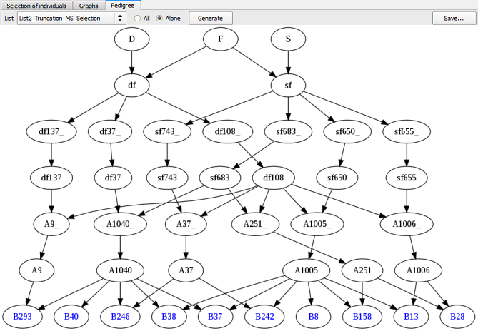
Figure 21: pedigree of individuals selected via the Truncation Selection method
It is possible to compare pedigrees coming from different lists of selection (see Fig. 21 & 22, Truncation Selection list vs. QCS, respectively). Note that the two individuals added via the QCS bring the parental allele x. So, if we use the QCS list to produce the next generation, the four parental alleles will be present in the next cycle.
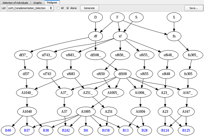
Figure 22: pedigree of individuals selected via the QCS method
This representation is useful to follow the contribution of selected individuals over generations of selection and to prevent possible bottlenecks (individuals coming from a reduced number of parents at a given generation), in order to limit risk of drift (which may lead for instance to the fixation of an undesired phenotypic type for traits not considered in the MARS process). It also can be used to maintain diversity for selection on traits complementary to those considered for the MARS process.